In-depth knowledge of scanning probe microscopy (SPM) dynamics is necessary when interpreting obtained images and especially when the sources of artifacts are to be identified. The aim of this research was to build and test the dynamic model of SPM electromechanical system. For simplicity reasons only atomic force microscopy (AFM) contact mode dynamics was explored.
The sensor part of AFM electromechanical system, most affecting the image quality, is subjected by the following forces: cantilever spring force, friction force, inertia and the force of interaction with the sample:
$$F_{inertia} + F_{spring} + F_{friction} = F(z); \tag{1}$$
The most simple approach, which nevertheless leads to a realistic description of most tip movements, is to start with Newton's equation of motion: [1,2]:
$$m\frac{\mathrm{d}^2 z}{\mathrm{d}t^2} + \gamma \frac{\mathrm{d}z}{\mathrm{d}t} + kz = F(z); \tag{2}$$
$m$ - the effective mass of the cantilever, $k$ - the spring constant of the cantilever, and $\gamma = 2\sqrt{\frac{k}{m}}$ - the dissipation term.
A linear second order differential equations is written as [3]:
$$\frac{\mathrm{d}^2 z}{\mathrm{d}t^2} + 2\xi \omega_n \frac{\mathrm{d}z}{\mathrm{d}t} + \omega_n^2 z = \omega_n^2 x \tag{3}$$
where $\omega_n = \sqrt{k/m}$ is the undamped angular frequency of the cantilever and $\zeta$ is a constant called the damping ratio.
The transfer function of (3) is[3]:
$$\frac{Z(s)}{X(s)} = \frac{\omega_n^2}{s^2 + 2\xi \,\omega_n s + \omega_n^2} \tag{4}$$
From (1), (2), (3) and (4), we obtain the transfer function, from which a model of Matlab/Simulink model was created (Fig. 1.).
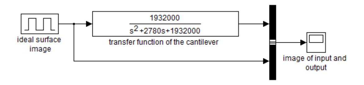
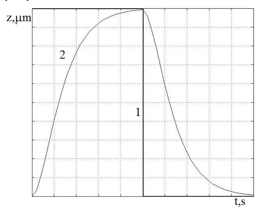
Rectangular 5 ms 1 μm hight pulses simulate the ideal surface profile. Coefficients were obtained by the manufacturer's data available on the Nanosurf EasyScan 2 SPM, working with CONTR cantilever. Coefficients obtained for a contact mode have following values: $k = 0.2N / m$, $b = 50\mu m$, $h = 2\mu m$, $l = 450\mu m$. On the Fig. 2 the system output is compared with an input. Dynamic errors can be explicitly observed.