In this work we seek to utilize the Frequency-Domain (FD) method [1] for the investigation of charge carrier transit in organic optoelectronic devices and to show that this technique is financially more appealing than other currently utilized methods, i.e. Time-of-Flight (TOF) [2] or Carrier Extraction by Linearly Increasing Voltage (CELIV) [3], both of which need expensive equipment capable of generating short impulses of light – lasers – as a prerequisite.
The TOF method is often called upon for determining charge carrier mobility and relaxation times in materials of small conductivity and mobility, solar cells. TOF's basis is applying a constant voltage U to a sample, exciting a layer of thickness d with a light impulse and then measuring the drift time $\tau$ of photogenerated charge carriers. The kinetics of the former frequently follows an exponential decay law, Eq. (1) and the carrier mobility $\mu$ can be determined appropriately, Eq. (2):
$$n(t) = n_0 e^{-t/\tau}\tag{1}$$$$\mu = d^2/U\tau\tag{2}$$where t - time, n0 – concentration of carriers at t = 0. Still, the small density of injected carriers leads to a low signal-to-noise ratio; this can be improved by using samples, which are grown in substrates of silicon, indium tin oxide (ITO) and etc. [4]
Knowledge about TOF is necessary to change parameters from FD into ones that describe a solar cell. These methods are bound by an inverse Fourier transform: in an FD procedure, the sample signal (i.e., photovoltage) decay time $\tau$ for an arbitrary frequency f is determined by knowing the phase shift $\varphi$ between two modulated excitation (modulation depth M) and sample response (mod. depth m) harmonic signals. For example, during mono-exponential decay: $\tan \varphi = 2\pi f \tau$, $\mu = m/M = (1 + \tan^2 \varphi)^{-0.5}$. (3)
In a more general case, whence decay is a weighted sum of several exponents, the FD method allows us to evaluate several different decay times $\tau_i$ that are influenced by the sample's structure specifics (having found the correct coefficients $a_i$):
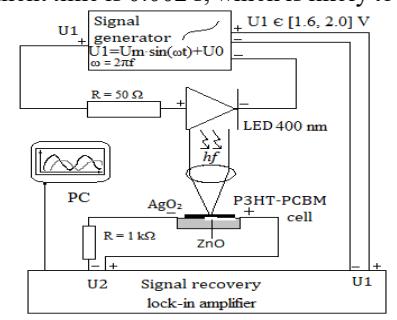
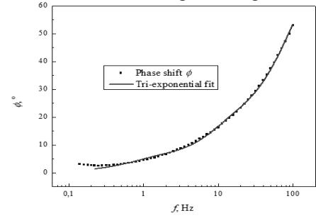
$$\tan \varphi = \frac{N_{\omega}}{D_{\omega}}, \ \mu = \frac{m}{M} = \sqrt{N_{\omega}^2 + D_{\omega}^2}, \ N_{\omega} = \frac{\sum_{i} \frac{a_{i} \omega \tau_{i}^2}{1 + \omega^2 \tau_{i}^2}}{\sum_{i} a_{i} \tau_{i}}, \ D_{\omega} = \frac{\sum_{i} \frac{a_{i} \tau_{i}}{1 + \omega^2 \tau_{i}^2}}{\sum_{i} a_{i} \tau_{i}}, \ \sum_{i} a_{i} = 1, \omega = 2\pi f.\tag{4}$$A block diagram regarding our experimental setup is presented in Fig. 1. We used a bulk heterojunction poly(3-hexilthiophene-2,5-diil)/[6,6]-phenil-C61 butyric acid (P3HT/PCBM) based photovoltaic material with transparent ZnO and Ag2O paste electrodes as the sample. This we expect slow drift times of orders 10-3 – 100 s. For the excitation we used a 3 mW 400 nm LED. The generator creates two identical phase-aligned harmonic signals, changing from 1.6 to 2 V, directed to a phase analyzer and the LED. The voltage range was chosen to not saturate the excitation or photovoltaic response signals and maintain their sinusoidal shape. The solar cell's contacts are connected to the phase analyzer: this way both the excitation and the modulated phase-shifted response signals are provided for comparison. The mentioned apparatus and generator are connected to a PC via USB; software controls the signals' frequency and executes logarithmic stepping over an arbitrary frequency interval. The final isolated (after removing system environmental noises) phase shift $\varphi$ between the excitation and photovoltaic response signals vs harmonic signal frequency f is shown in Fig. 2. Applying a tri-exponential decay fit to our sample yielded the following decay durations $\tau_i$ and their appropriate weights $a_i$: $\tau_1 = 0.002$ s, $a_1 = 0.91$; $\tau_2 = 0.012$ s, $a_2 = 0.08$ and $\tau_3 = 0.112$ s, $a_3 =0.01$. It is evident that our calculated values fall within the expected time range of 10-3 – 100 s and the most prominent time is 0.002 s, which is likely to play the most significant role when determining the charge carrier's mobility.