Since 2018 in Baldone Observatory around 50 new asteroids were discovered and for more than 6000 asteroids astrometric positions were published in MPC circulars. For many asteroids, there are physical properties that have not been analyzed and calculated yet, including one of the most important – the rotation period.
To get the rotation period, time-resolved photometry is needed for each of the asteroids, which can be used to acquire the light curve of the object. To get a precision of $0.03^m$ for measurments, the following was done: each sky region was observed at least from 3 to 5 nights. To process the images, flats, bias, and dark calibration images were taken each night. The program "MaxIm DL 5" was used to reduce and align the images. The flat-field images were taken against the twilight sky. The exposure time for dark images was the same as for respective light images – two or three minutes for all asteorids. Position measurements were made with the help of "Astrometrica", the new genesis of the program "CoLiTec" ("Lemur" [1]) and "Sky Sift" [2] programs. The brightness measurements were made with "MaxIm DL 5" or "Lemur". The program 'Lemur' was used to perform differential photometry on the reduced data. For each data set, more than five stars were used for brightness comparison to the asteroid. Aperture photometry using a differential photometry technique was done to determine the brightness of comparison stars and the asteroid in GAIA G(RP) passband.
A standardized methodology is used to process the luminosity curves to eliminate differences in observations over time. For example, data from all series of observations are reduced to a single epoch, usually to the first series of observations. For brightness, two adjustments are made – related to distance and phase - to change all measurements to the first series of observations.
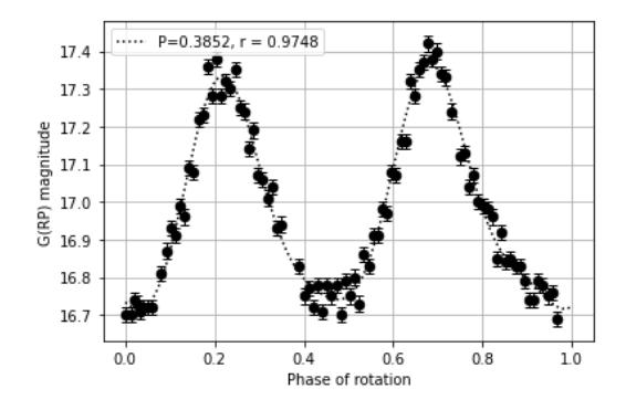
After the data has been processed, a program made in Python is used to get the rotation period with Fourier series analysis. A simple version of rotation around a single axis is showed in Eq.(1):
$$V_r = A_0 + \sum_{i=1}^n B_n \sin\left(\frac{2\pi n \theta}{P}\right) + \sum_{i=1}^n C_n \cos\left(\frac{2\pi n \theta}{P}\right),\tag{1}$$where $V_r$ is the appearant magnitude, $A_0$, $B_n$, $C_n$ are Fourier constants, P is the period and t is the time in Julian days. The algorithm works with itterating through intial guesses two times with different time steps for the period and searching for the best fit for the light curve. In the end the acquired period is visualized as in Fig. 1.