Singlet-singlet annihilation is a common phenomenon in molecular structures. It is often difficult to provide experimental conditions that could prevent annihilation – the excitation radiation of low intensity must be used, so that at most one light photon per excitation pulse is absorbed per molecular aggregate, generating just a single electronic excitation. Consequently, to increase signal-to-noise ratio, the measurement time must be extended. These experimental conditions may not be suitable for some samples; therefore, it might often be necessary to account for annihilation while analyzing data.
Simple annihilation model can be described by rate equation Eq. 1:
$$ \frac{\mathrm{d}n}{\mathrm{d}t} = -\gamma n^2. \tag{1} $$here $n(t)$ is the mean number of remaining excitations in the system at time $t$ and $\gamma$ is the rate constant for annihilation. In this model, the size of molecular aggregate, excitation transfer rate across the aggregate, and initial population of excitations are considered very large. In order to include finite transfer rate, $\gamma$ must be considered as a function of time which at longer times can be approximated by a power law [1]. More precise modelling would also include discrete number of excitations, resulting in the system of Pauli Master equations [2].
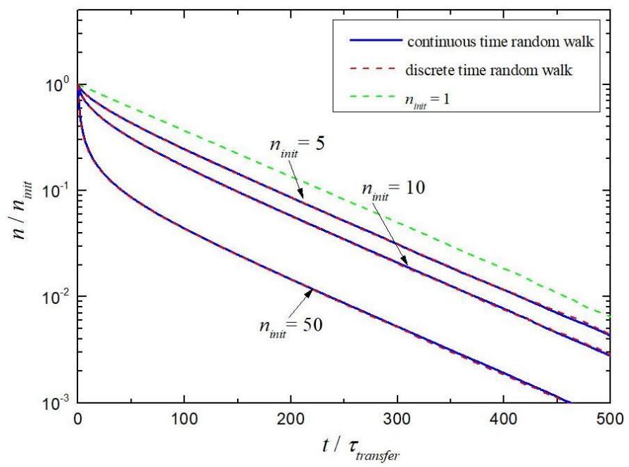
To account for both finite transfer rate and discrete number of excitations in annihilation model, we have chosen to use Monte Carlo method. During the modelling process one-dimensional molecular lattice is formed and excitations are randomly distributed in the lattice. At each time step, the excited state has three fates: it can stay in the same position, relax to the ground state, or move to another position with probability to annihilate if that site is already occupied. The fate is decided by generating random numbers. Eventually, number of excitations in the lattice becomes zero, and then the same process is repeated by generating new initial distribution. After 10 000 lattices have been generated, the average kinetics is calculated (Fig. 1). The first model was based on discrete time random walk. The same model is now modified and based on continuous time random walk. This modification reduces the computing time approximately ten times.